After a period of slow ice loss in the middle of June, Arctic sea ice loss ramped up, and extent at the end of the month fell below 2012, the year which ended up with the lowest September ice extent in the satellite record. A pattern of atmospheric circulation favored ice loss this June, which was also characterized by above average temperatures over most of the Arctic Ocean, and especially in the Laptev and East Siberian Seas.
Overview of conditions
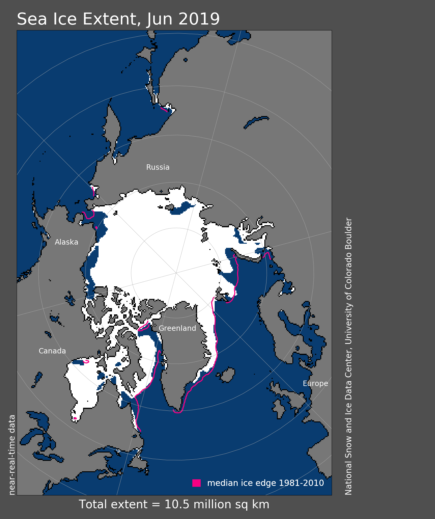
Figure 1. Arctic sea ice extent for June 2019 was 10.53 million square kilometers (4.07 million square miles). The magenta line shows the 1981 to 2010 average extent for that month. Sea Ice Index data. About the data Credit: National Snow and Ice Data Center
Arctic sea ice extent for June averaged 10.53 million square kilometers (4.07 million square miles). This is 1.23 million square kilometers (475,000 square miles) below the 1981 to 2010 average and 120,000 square kilometers (46,300 square miles) above the previous June record low set in 2016. Extent at the end of the month remained well below average on the Pacific side of the Arctic, with open water extending from the Bering Strait, and along the coasts of the Chukchi and Beaufort Seas all the way to Melville Island in the Canadian Arctic Archipelago. Sea surface temperatures (SSTs) in the open waters have been unusually high, up to 5 degrees Celsius (9 degrees Fahrenheit) above average in the Chukchi Sea, as indicated by the National Oceanic and Atmospheric Administration (NOAA) SST data provided on the University of Washington Polar Science Center UpTempO website. Large areas of open water are now apparent in the Laptev and Kara Seas with extent below average in Baffin Bay and along the southeast coast of Greenland.
Extent over the first 10 days of the month dropped quickly but then the loss rate suddenly slowed. From June 12 through June 16, extent remained almost constant at 10.8 million square kilometers (4.17 million square miles). Following this hiatus, extent then dropped fairly quickly through the remainder of the month. Overall, sea ice retreated almost everywhere in the Arctic in June. Exceptions included the northern East Greenland Sea, southeast of Svalbard, near Franz Joseph Land, and in the southeastern part of the Beaufort Sea, where the ice edge expanded slightly.
Conditions in context
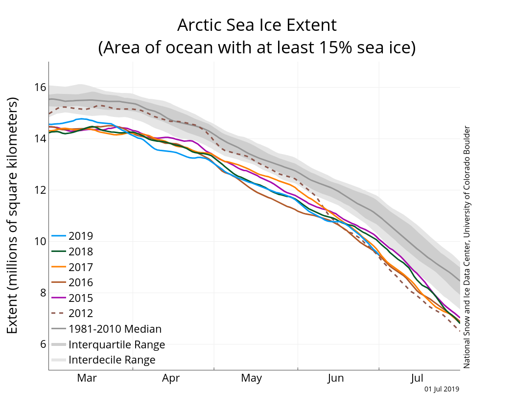
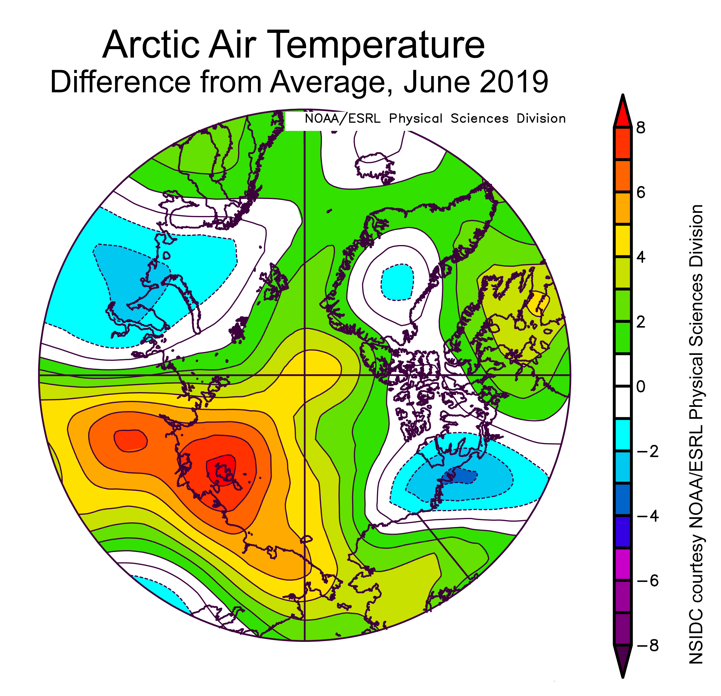
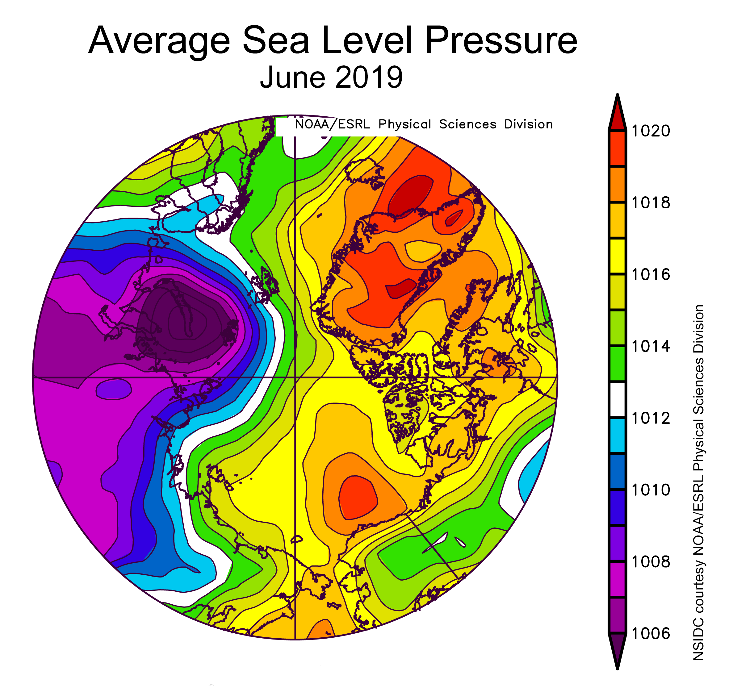
Figure 2a. The graph above shows Arctic sea ice extent as of July 1, 2019, along with daily ice extent data for four previous years and the record low year. 2019 is shown in blue, 2018 in green, 2017 in orange, 2016 in brown, 2015 in purple, and 2012 in dotted brown. The 1981 to 2010 median is in dark gray. The gray areas around the median line show the interquartile and interdecile ranges of the data. Sea Ice Index data. Credit: National Snow and Ice Data CenterFigure 2b. This plot shows the departure from average air temperature in the Arctic at the 925 hPa level, in degrees Celsius, for June 2019. Yellows and reds indicate higher than average temperatures; blues and purples indicate lower than average temperatures. Credit: NSIDC courtesy NOAA Earth System Research Laboratory Physical Sciences DivisionFigure 2c. This plot shows average sea level pressure in the Arctic in millibars (hPa) for June 2019. Yellows and reds indicate high air pressure; blues and purples indicate low pressure. Credit: NSIDC courtesy NOAA Earth System Research Laboratory Physical Sciences Division
Following May’s theme, air temperatures at the 925 hPa level (about 2,500 feet above the surface) in June were above the 1981 to 2010 average over most of the Arctic Ocean. However, the spatial patterns between the two months were different. While in May, it was particularly warm compared to average over Baffin Bay and a broad area north of Greenland, in June the maximum warmth of more than 6 to 8 degrees Celsius (11 to 14 degrees Fahrenheit) shifted to the Laptev and East Siberian Seas (Figure 2b). It was slightly cooler than average over the northern Barents and Kara Seas and over central Greenland and the western Canadian Arctic.
The atmospheric circulation at sea level featured high pressure over the north American side of the Arctic, with pressure maxima over Greenland and in the Beaufort Sea, paired with low pressure over the Eurasian side of the Arctic, with the lowest pressures over the Kara Sea (Figure 2c). This pattern drew in warm air from the south over the Laptev Sea where temperatures were especially high relative to average. This circulation pattern bears some resemblance to the Arctic Dipole pattern that is known to favor summer sea ice loss, which was particularly well developed through the summer of 2007. So far, the pattern for the 2019 melt season is very different than the past three years, which featured low pressure over the central Arctic Ocean.
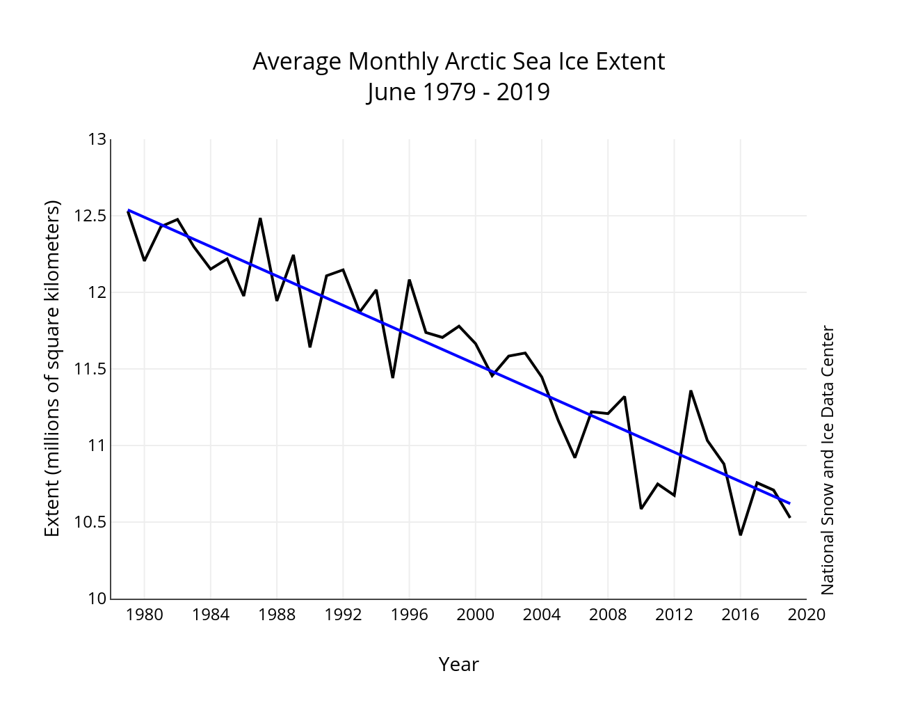
Figure 3. Monthly June ice extent for 1979 to 2019 shows a decline of 4.08 percent per decade. Credit: National Snow and Ice Data Center
June 2019 compared to previous years
The average extent for June 2019 of 10.53 million square kilometers (4.07 million square miles) ended up as the second lowest in the satellite record. The current record low of 10.41 million square kilometers (4.02 million square miles) was set in June 2016. Overall, sea ice extent during June 2019 decreased by 2.03 million square kilometers (784,00 square miles). Because of the fairly slow loss rate near the middle of the month, the overall loss rate for June ended up being fairly close to the 1981 to 2010 average. The linear rate of sea ice decline for June from 1979 to 2019 is 48,000 square kilometers (19,00 square miles) per year, or 4.08 percent per decade relative to the 1981 to 2010 average.
Sea Ice Outlook posted for June
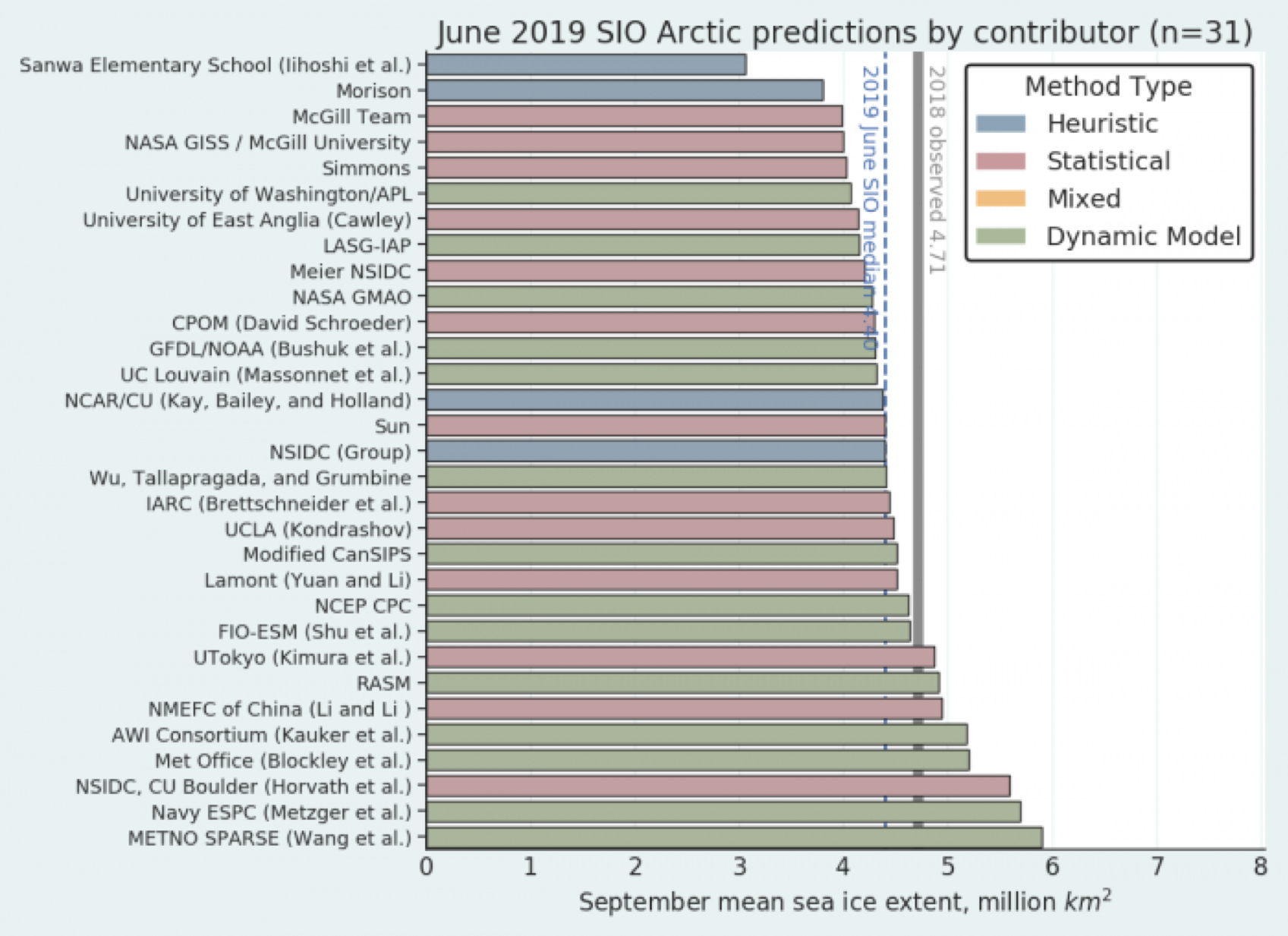
Figure 4. This chart shows the projections of total Arctic sea ice extent based on conditions in May from 31 contributors. Credit: Sea Ice Prediction Network
The Sea Ice Prediction Network–Phase 2 recently posted the 2019 Sea Ice Outlook June report. This report focuses on projections of September sea ice extent based on conditions in May. The projections come variously from complex numerical models to statistical models to qualitative perspectives from citizen scientists. There were 31 contributions for projected total Arctic sea ice extent and of these 31, nine also provided projections for extent in Alaska waters, and six provided projections of total Antarctic extent (Figure 4). There were also seven predictions of September extent for Hudson Bay.
The median of the projections for the monthly mean September 2019 total Arctic sea ice sea-ice extent is 4.40 million square kilometers (1.70 million square miles) with quartiles (including 75 percent of the 31 projections) of 4.2 and 4.8 million square kilometers (1.62 and 1.85 million square miles). The observed record low September extent of 3.6 million square kilometers (1.39 million square miles) was set 2012. Only three of the projections are for a September 2019 extent below 4.0 million square kilometers (1.54 million square miles) and only one is for a new record at 3.06 million square kilometers (1.18 million square miles).
Thicker clouds accelerate sea decline
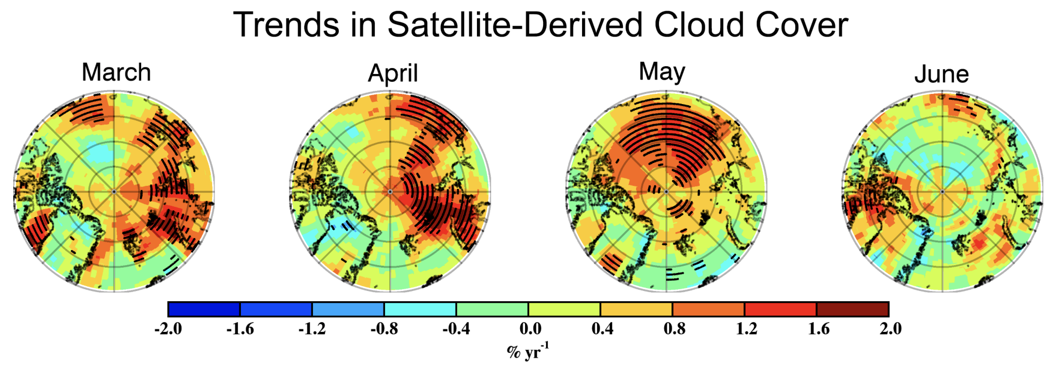
Figure 5. These plots show linear trends of satellite-retrieved cloud cover, percent per year, for March through June over the Arctic (70 to 90 degrees North) from 2000 to 2015. Blues depict declines in cloud cover while reds depict increases. Cloud observations are derived from CERES-MODIS SYN1 Ed3.0 product.
A new study led by Yiyi Huang of the University of Arizona presents evidence of a link between springtime cloud cover (Figure 5) over the Arctic Ocean and the observed decline in sea ice extent. Based on a combination of observations and model experiments, there may be a reinforcing feedback loop. As sea ice melts, there is more open water which promotes more evaporation from the surface and hence more water vapor in the atmosphere. More water vapor in the air then promotes the development of more clouds. This increases the emission of longwave radiation to the surface, further fostering melt. The process appears to be effective from April through June. But since the atmosphere influences the sea ice and the sea ice influences the atmosphere, separating cause and effect remains unclear.
Antarctic sea ice at record low for June
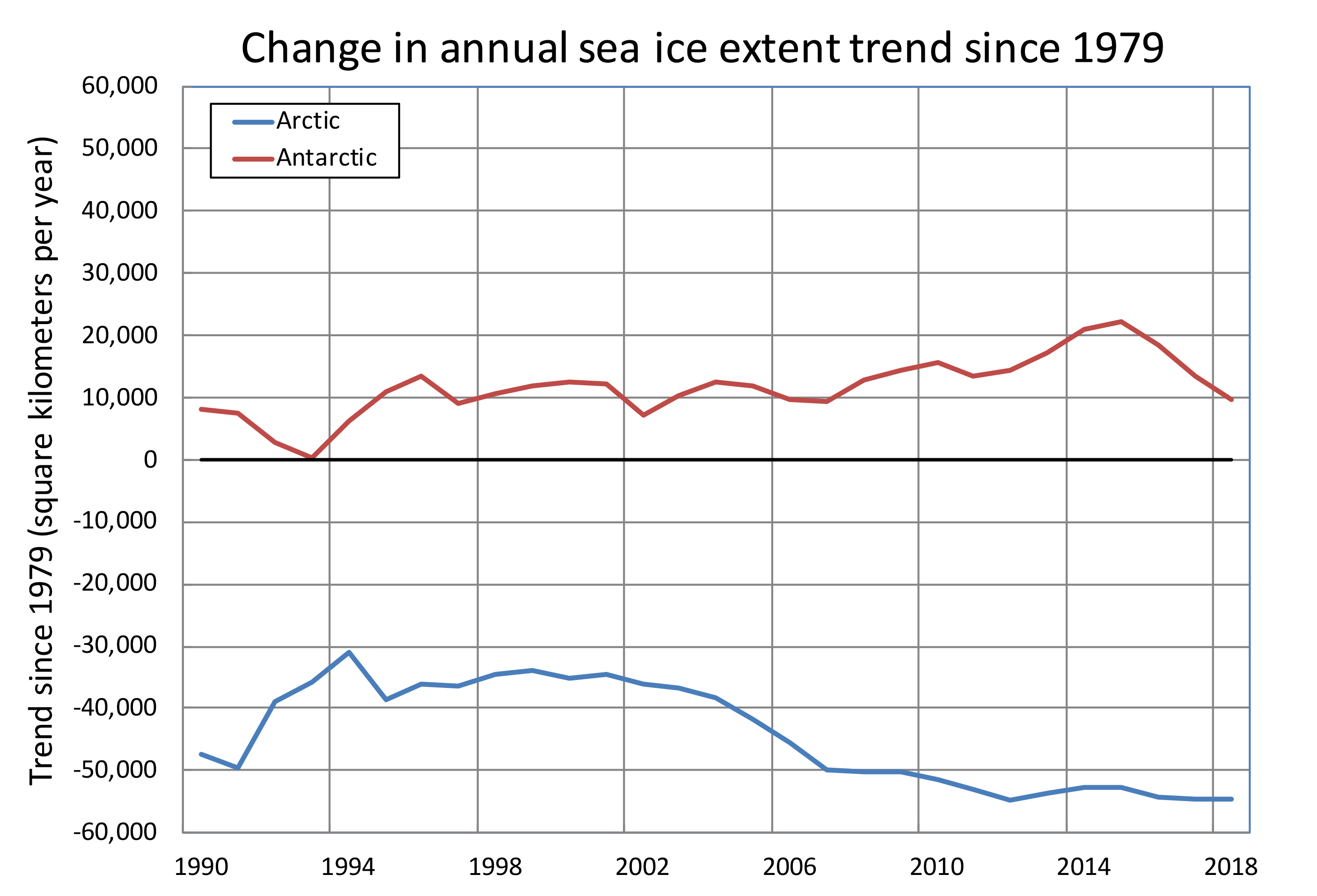
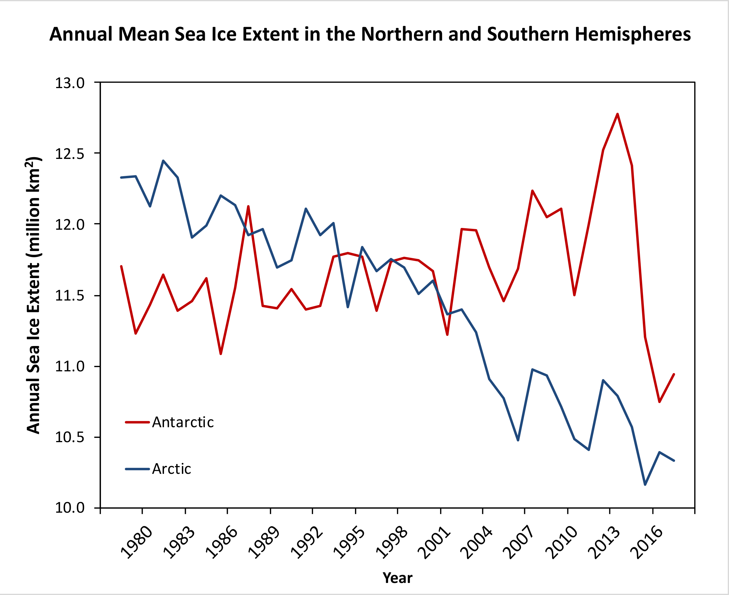
Figure 6a. This plot shows the evolution of linear trends in annual average sea ice extent for the Arctic, in blue, and Antarctic, in red. The trend was first computed from 1979 through 1990, then from 1979 through 1991, then 1979 through 1992, and so on. Even with the recent declines in Antarctic sea ice extent, the linear trend is still slightly positive. The reason for starting the trend calculation from 1979 through 1990 is that it provides a sufficient number of years to compute a trend. Credit: W. Meier, NSIDCFigure 6b. This plot shows the average annual sea ice extent from 1979 through 2018 in the Arctic, in blue, and Antarctic, in red, from the Sea Ice Index using the NASA Team sea ice algorithm. Credit: J. Stroeve, NSIDC
Sea ice surrounding Antarctica was at the lowest mean monthly extent for June, surpassing 2002 and 2017. At the month’s end, sea ice averaged approximately 160,000 square kilometers (62,000 square miles) below the previous record low set in 2002, and over 1.1 million square kilometers (425,000 square miles) below the 1981 to 2010 average. Ice extent was particularly low in the eastern Weddell Sea and the region north of Enderby Land (south of the western Indian Ocean), and north of eastern Wilkes Land. No region had substantially above average sea ice extent in June.
A new paper published by our colleague Claire Parkinson at NASA Goddard Space Flight Center (GSFC) discusses the large drop in Antarctic sea ice extent between 2014 and 2017. The winter maximum for 2014 was unusually high, setting the 40-year record maximum extent. Our earlier posts noted the dramatic recent decline, particularly in the austral spring of 2016. Sea ice has remained below the 1981 to 2010 reference period extent since late 2016.
While the recent decline is noteworthy, trends in Antarctic sea ice extent over the continuous satellite record since late 1978 remain slightly positive (Figure 6a). Antarctica experiences large inter-annual variability because of its unconfined geography—open to the Southern Ocean on all sides—and strong influences of the varying Southern Annular Mode pattern of atmospheric circulation. Sparse satellite data from the 1960s indicate large swings in that decade as well. Previous studies have attributed the onset of the recent decline as a response to a series of intense storms. Unlike Arctic sea ice extent, which evinces a longterm downward trend, Antarctic sea ice extent displays enormous variability that is natural for the southern sea ice system (Figure 6b). Thus, a clear climate-related signal cannot yet be discerned for sea ice in the southern hemisphere.
From the Associated Press via The Greeley Tribune:
A company that operates a historic railroad that carries tourists through southwestern Colorado’s mountains and forests was accused Tuesday in a lawsuit of causing one of the largest wildfires in state history.
Federal investigators found that a coal-burning engine operated by the Durango & Silverton Narrow Gauge Railroad and American Heritage Railways threw cinders or other hot material onto brush near its track and started a fire on June 1, 2018, according to the office of U.S. Attorney Jason Dunn.
Flames eventually consumed about 85 square miles (220 square kilometers) of land near Durango, prompting evacuation orders affecting hundreds of people. Much of the damage occurred in the San Juan National Forest and on other federal land…
Officials had not disclosed a cause of the fire before Dunn’s office filed the lawsuit, which says multiple eyewitnesses told federal investigators that one of the trains passed through the area immediately before the fire began…
Residents and businesses have filed their own lawsuit against the railroad company, arguing that it knew or should have known about drought conditions that summer.
A statement released by Dunn’s office said federal authorities estimated damage and fire suppression involving the blaze could hit $25 million.
“This fire caused significant damage, cost taxpayers millions of dollars, and put lives at risk,” Dunn said in a statement. “We owe it to taxpayers to bring this action on their behalf.”
The 416 Fire near Durango, Colorado, ignited on June 1, 2018. By June 21, the wildfire covered more than 34,000 acres and was 37 percent contained. Photo credit USFS via The High Country News
416 Fire July 2, 2018. Graphic credit Incweb
The 416 Fire started at about 10 a.m. on June 1, 2018, approximately 10 miles north of Durango, CO. Rocky Mountain Type 1 Incident Management Team is managing the fire. The fire is burning on the west side of State Highway 550 on some private land and on the San Juan National Forest. The fire is burning in grass, brush, and timber. The Weather conditions remain critical and fuels are ideal for significant fire growth. The fire has been very active and continues to burn in rough and inaccessible terrain. Many homes have been evacuated and structure protection is in place. Map via Inciweb
Screen shot of Animas River debris flow July 2018 aftermath of 416 Fire (CBS Denver).
Debris flow from 416 Fire. Photo credit: Twitter #416Fire hash tag
The Lower Colorado River Basin does not avoid a shortage in 2020 despite the plentiful snowpack on the Rocky Mountains this past winter.
Why? Well, the new Drought Contingency Plan defines different “tiers” of shortage. The Lower Basin will not drop into a Tier One shortage next year because Lake Mead will almost certainly remain above 1,075 feet in elevation.
At the same time, Mead will likely remain under 1,090 feet. That triggers a Tier Zero shortage.
“Under Tier Zero conditions, Arizona takes a reduction of 192,000 acre-feet in its annual Colorado River entitlement,” said Suzanne Ticknor, assistant general manager at the Central Arizona Project…
Arizona’s reduced supply in Tier Zero will affect certain users of the Central Arizona Project canal system. There will be a slight reduction to some Pinal County farmers, and the pool of so-called “excess water” will be eliminated.
Regular buyers of excess water have included the United States, the Arizona Water Banking Authority and the agency that replenishes groundwater in Central Arizona, which enables new home building.
The CAP is writing a new policy for excess water if and when it returns.
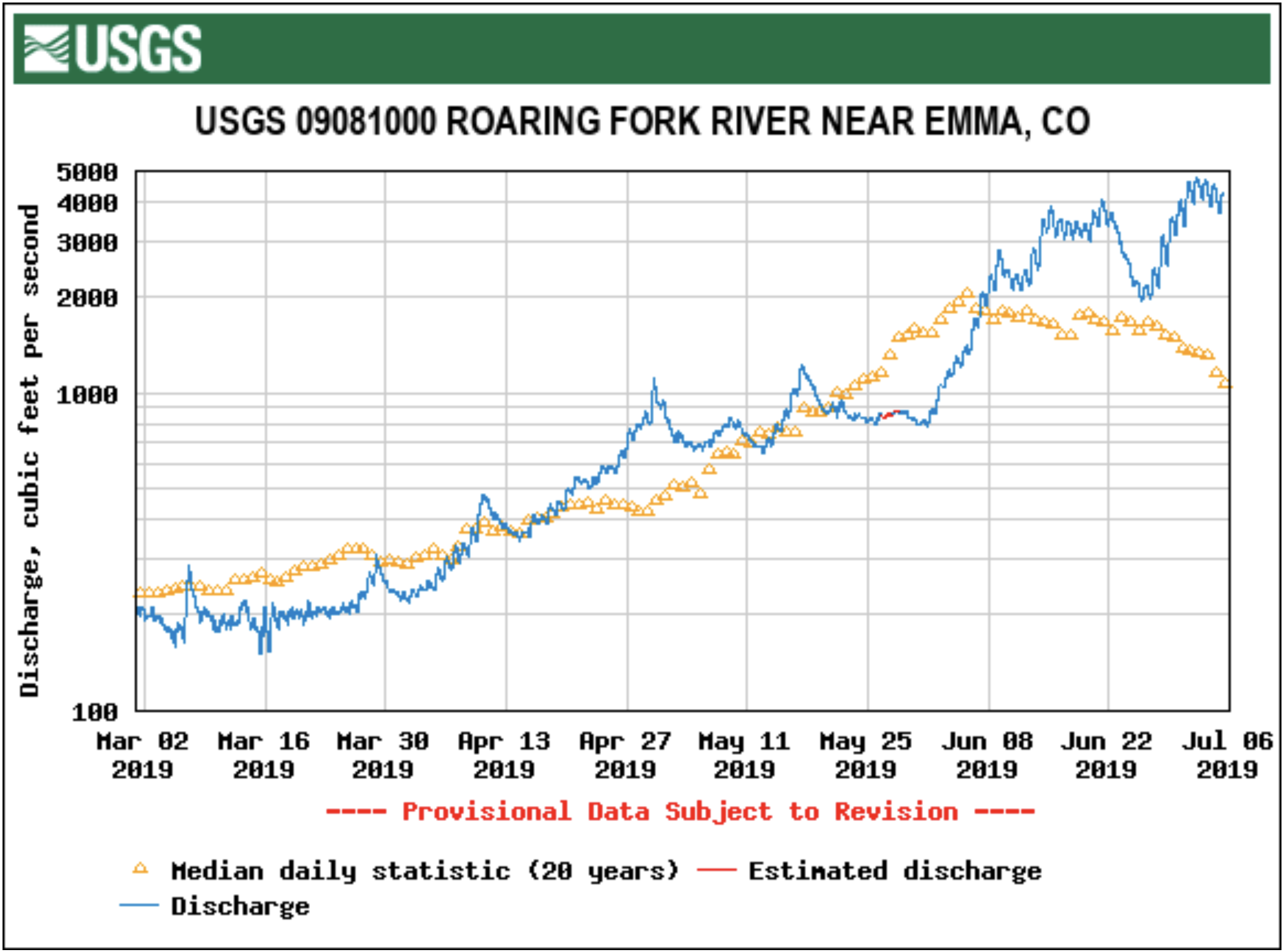
A flood advisory has been issued for all major rivers in the Roaring Fork watershed by the National Weather Service. The advisory is in effect until further notice.
According to a report issued Wednesday by the Roaring Fork Conservancy, the rivers in this watershed are currently flowing at more than twice the average for this time of year.
On Monday, the Roaring Fork River at Glenwood Springs hit 9,030 cubic feet per second, which is the biggest peak of 2019, according to RFC’s report. While flows have declined slightly since July 1, they are expected to surge over the next week, the report continued.
The Fryingpan River below Ruedi Reservoir was measured at 950 cfs on Wednesday, according to the RFC.
Basalt Police Chief Greg Knott said in his six years at the helm, he’s seen the Fryingpan River hit 950 cfs just one other time, which was in 2016.
Both Ruedi and Twin Lakes reservoir are expected to fill to capacity in the coming days.
“These elevated flows will cause the Fryingpan River to remain above bankfull levels,” according to the NWS. “Minor lowland flooding can be expected along the river.”
[…]
The July 3 report from RFC showed the Roaring Fork River in Aspen at 747 cfs and at a whopping 4,370 cfs in Basalt below the confluence with the Fryingpan River.
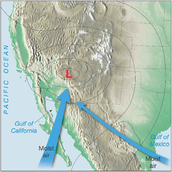
Southwest Colorado appears to be headed into a dry spell, and even the monsoon may be drier than average, according to the National Weather Service…
The onset of the monsoon, which usually arrives in mid-July, appears to be arriving later than usual, said Chris Sanders, a meteorologist with NWS.
“Typically, we look for a big ridge of high pressure to set up over the center part of the U.S.,” Sanders said. “That’s the most favorable pattern to get moisture to come up into the area. Right now, we’re seeing the exact opposite, where we’re having troughing coming into that area.”
Sanders said troughing can lead to drier air and shuts off the feed of moisture needed to produce afternoon storms in Southwest Colorado.
The pattern has the potential to remain stagnant going into August, but there may be some surges of moisture. It depends on what happens with the high-pressure ridge over the West Coast. Where exactly the ridge sets up will play a role in the possibility of moisture being pulled from the coast into the Intermountain West.
Sanders said it is difficult to determine when the monsoon will arrive, but typically, the monsoon starts during early to mid-July.